Color Quantization

May 20, 2024

To inaugurate this blog, I'd like to present a simple article involving a topic I've spent many months studying: clustering. While the application to color quantization is not complicated, it will serve as an excuse to show off the fancy formatting and data visualization tools I've included in this site.

Let's inspect the following image:

Brachyscome iberidifolia [ 1 ]

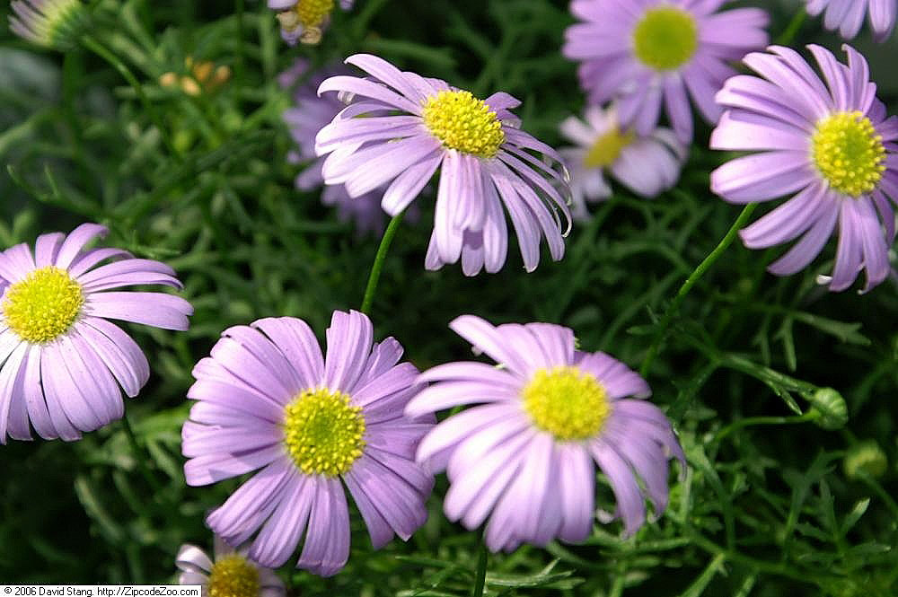
If you were asked to list the prominent colors in this image, how would you respond? At a minimum, I would identify:

Green (background foliage)
Light Violet (flower petals)
Yellow (flower centers)

Fundamentally, this image is an array of pixels. The color of each pixel is described by a combination of three integers, each in the range 0-255. You know this as RGB color encoding. Pure black is encoded as (0,0,0) and pure white as (255,255,255).

Knowing this, we can determine the number of unique colors in this image by counting the number of unique RGB triplets:

python

import requests
from PIL import Image
from io import BytesIO
import numpy as np
 
url = 'https://upload.wikimedia.org/wikipedia/commons/f/f2/Brachyscome_iberidifolia_Toucan_Tango_2zz.jpg'
 
# Wikimedia access requires a user agent
headers = {
    'User-Agent': 'DataDiary/0.1 ([email protected])'
}
response = requests.get(url, headers=headers)
image = Image.open(BytesIO(response.content))
image = image.convert('RGB')
 
image_array = np.array(image)
height = image_array.shape[0]
width = image_array.shape[1]
image_array_flat = image_array.flatten().reshape((
    height * width,
    3
))
 
view = image_array_flat.view((
    np.void,
    image_array_flat.dtype.itemsize * image_array_flat.shape[1]
))
num_colors = len(np.unique(view))
 
print(image_array_flat.shape, num_colors)

This reports 665,000 pixels with 141,862 unique colors. More than you thought, right? What if we were operating under strict storage/bandwidth limitations? Could we devise a simple compression technique to reduce the size of this image while maintaining the original resolution? You already employed a clever strategy at the beginning of this article: reduce the diverse color space to a handful of prominent representative colors.

K-Means Clustering

How can we algorithmically identify the most faithful representatives of our color space? A simple solution is K-Means clustering. We start by choosing the number of colors to appear in our compressed image, n. We randomly cast out n points, called centroids, into the color space. Then, we repeatedly run the following two steps to guide the centroids to popular pockets of the space:

Assign each point (pixel) to the nearest centroid.
Move each centroid to the mean position of the points that are currently assigned to it.

The animation below shows three centroids gravitating to three natural clusters with this simple logic:

K-means convergence animation with 3 centroids

K-means convergence [ 2 ]

Let's give this a try on our image. We configure K-Means with 3 centroids and iterate until convergence. We then replace the color of each pixel with the color of the nearest centroid:

python

def KMeans(X, n_clusters, max_iter=100, tol=1e-4):
    # initialize centroids at positions of random pixels
    centroids = X[np.random.choice(X.shape[0], n_clusters, replace=False)]
 
    for _ in range(max_iter):
        # assign each pixel to the nearest centroid
        distances = np.linalg.norm(X[:, np.newaxis] - centroids, axis=2)
        labels = np.argmin(distances, axis=1)
 
        # update each centroid to the mean of assigned pixels
        new_centroids = np.array([X[labels == k].mean(axis=0) for k in range(n_clusters)])
 
        # check for convergence
        if np.all(np.linalg.norm(new_centroids - centroids, axis=1) < tol):
            break
 
        centroids = new_centroids
 
    return centroids, labels
 
n_clusters = 3
centroids, labels = KMeans(image_array_flat, n_clusters)
centroids = np.round(centroids)
 
# replace pixels with representative centroids
quantized_image_array_flat = centroids[labels]
 
quantized_image_array = quantized_image_array_flat.reshape(image_array.shape)
quantized_image = Image.fromarray(quantized_image_array.astype('uint8'), 'RGB')
 
quantized_image.save('Brachyscome_iberidifolia_Toucan_Tango_2zz_KMEANS3.png', 'PNG')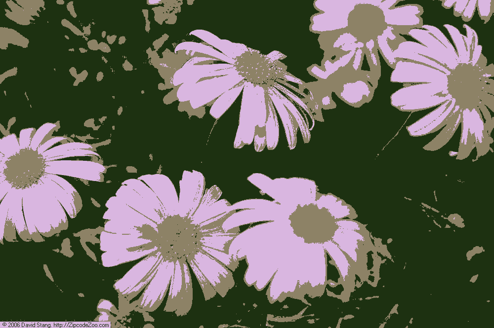

Brachyscome iberidifolia after K-means quantization with 3 centroids

A pale imitation. What happened here? We can visualize the final positions of the centroids in the color space to better understand this result:

python

import plotly.graph_objects as go
 
# sample 10k pixels to appear in the visual
image_array_flat_sample = image_array_flat[np.random.choice(image_array_flat.shape[0], 10_000)]
 
# plot pixels
fig = go.Figure(data=[go.Scatter3d(
    x=image_array_flat_sample[:, 0],
    y=image_array_flat_sample[:, 1],
    z=image_array_flat_sample[:, 2],
    mode='markers',
    marker=dict(
        size=1.5,
        color=[f'rgb({pixel[0]}, {pixel[1]}, {pixel[2]})' for pixel in image_array_flat_sample],
        opacity=1.0,
        line=dict(width=0)
    ),
    hovertemplate = '<b>R</b>: %{x}<br><b>G</b>: %{y}<br><b>B</b>: %{z}<extra></extra>',
    showlegend=True,
    name='pixels'
)])
 
# plot centroids
fig.add_trace(go.Scatter3d(
    x=centroids[:, 0],
    y=centroids[:, 1],
    z=centroids[:, 2],
    mode='markers',
    marker=dict(
        size=8,
        color=[f'rgb({centroid[0]}, {centroid[1]}, {centroid[2]})' for centroid in centroids],
        opacity=1.0,
        symbol='x',
        line=dict(width=0)
    ),
    hovertemplate = '<b>R</b>: %{x}<br><b>G</b>: %{y}<br><b>B</b>: %{z}<extra></extra>',
    showlegend=True,
    name='centroids'
))
 
fig.update_layout(
    uirevision='constant',
    scene=dict(
        xaxis=dict(title='R', showspikes=False, range=[0, 255]),
        yaxis=dict(title='G', showspikes=False, range=[0, 255]),
        zaxis=dict(title='B', showspikes=False, range=[0, 255])
    ),
    scene_aspectmode='manual', 
    scene_aspectratio=dict(x=1, y=1, z=1)
)
 
with open('centroids_in_color_space.json', 'w') as outfile:
    outfile.write(fig.to_json())

Drag to rotate and scroll to zoom. Use the legend on the right to disable the pixel markers and reveal the obscured centroids.

With only 3 centroids, it appears that some regions are left without a close representative. Light violet and dark green are well-served, but notice the empty pocket of yellow. What if we try again with 10 centroids?

Brachyscome iberidifolia after K-means quantization with 10 centroids

Much better. Additional centroids will yield diminishing returns, so let's call this a victory.

Attributions

Brachyscome iberidifolia by David Stang, licensed under CC BY-SA 4.0.
Source: Wikimedia Commons
Modifications: Cropped and resized
K-means convergence by Chire, licensed under GNU Free Documentation License.
Source: Wikimedia Commons