Bayesian Optimization for Vehicle Control

I was looking for introductory material on Bayesian optimization and found this helpful paper: "A Tutorial on Bayesian Optimization of Expensive Cost Functions, with Application to Active User Modeling and Hierarchical Reinforcement Learning". Quite a mouthful. In it, the authors run an experiment where they train a virtual car to take a clean U-turn at a fixed speed using the following control network:

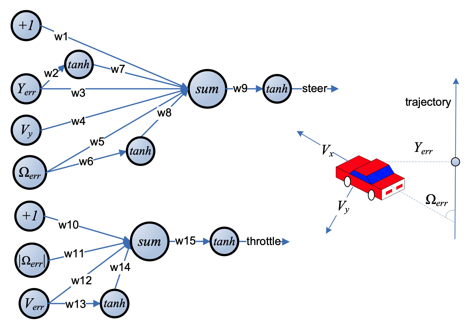
You can see how, at any given time, the car's throttle and steering are goverened by 4 measurements:

1. The lateral distance between the car and the road, $Y_{err}$
2. The angle between the car's heading and the the road direction, $\Omega_{err}$
3. The difference between the desired speed of the car and the current speed, $V_{err}$
4. The lateral velocity of the car relative to its own heading (a.k.a. "drift"), $V_y$

These are filtered through a total of 15 weights (in combination with summation and tanh squashing) to produce two values in range (-1, 1). The goal is to come up with a set of weights that encourages the car to stay on the road without deviating too much from a fixed speed through the duration of the turn.

Let's set up our own simulation and give this a try!

Background: Bayesian Optimization

So, why do the authors propose this problem as a candidate for Bayesian optimization? Two reasons:

1. We don't know the shape of the reward function a priori. We have to propose a set of weights, send the car through the U-turn, then calculate the reward at the end of the trial.
2. The reward is expensive to evaluate. We can't afford to probe the entire 15-dimensional parameter space when each trial requires a real-time simulation.

Bayesian optimization introduces two constructs to address these challenges: the surrogate function and the acquisition function. The simplest way to explain their interplay is to walk through a demo of the optimization of just 1 parameter.

Let's say we've already conducted 5 trials and plotted the reward values:

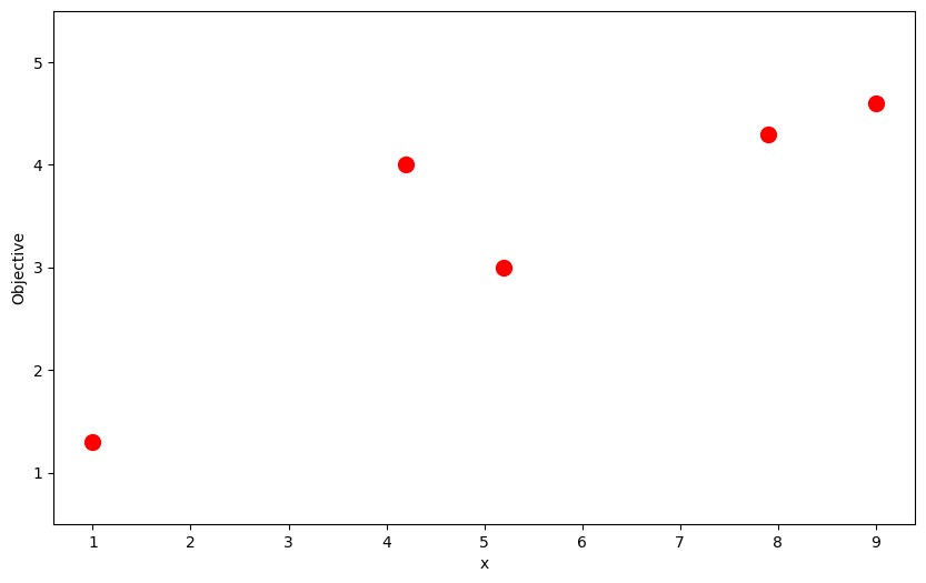
Where should we conduct the next trial? We're blind to the function that generated these points. However, we can try to estimate the shape of the function in a manner that leverages the information we've gathered. This is where we apply a surrogate function:

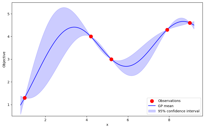
This "function" is actually a Gaussian Process - a distribution over infinitely many functions. It's characterized by its mean (solid line) and uncertainty (transparent envelope). Notice how its mean passes directly through our observations and how its envelope grows as it steers through uncharted territory. This reflects our confidence in the estimation of the true function near the observations and our uncertainty in regions where there is little information upon which to extrapolate. In this example, I've defined it with the Scaled RBF kernel:

If you'd like to learn exactly how a kernel can define the shape of a GP, I encourage you to visit the paper that inspired this article.

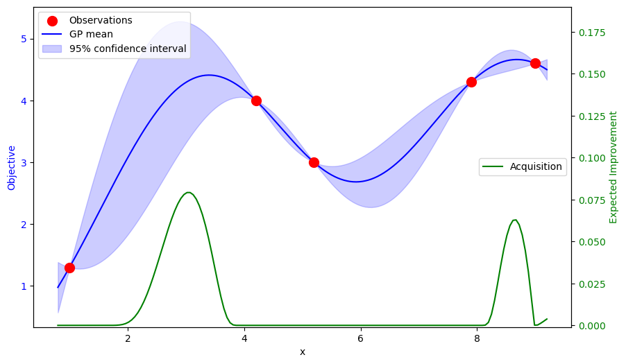
Now, we have to decide where to conduct our next trial based on the surrogate. It predicts a low-uncertainty peak near the rightmost observation. However, it appears that the high-uncertainty region on the left has the potential to yield an even greater reward. We need a mechanism that can incorporate both of these considerations to estimate the improvement we can expect to observe at any point in the domain. This is where an acquisition function can help. Here, I've chosen to implement the aptly-named Expected Improvement function:

Where:

• $\mu(x)$ is the mean of the GP at point $x$
• $f(x^+)$ is the best reward value so far
• $\sigma(x)$ is the standard deviation at point $x$
• $Z = \frac{\mu(x) - f(x^+) - \xi}{\sigma(x)}$
• $\Phi$ is the CDF of the standard normal distribution
• $\phi$ is the PDF of the standard normal distribution
• $\xi$ is an exploration-exploitation tradeoff parameter

You'll notice that this expression is a sum of two terms. The first is the exploitation term. It says: "look for points where the mean of the GP is greater than the best observation with little uncertainty". This is the main contribution to the peak on the right. The second term is the exploration term. It says: "look for points where large uncertainty permits a high probability of exceeding the best observation". This drives the peak on the left. Also, note the tradeoff parameter, $\xi$. This allows us to adjust the balance of the terms to create a more/less adventurous optimizer.

My choice of $\xi$ has resulted in a peak around $x=3$, so this is where we would conduct the next trial and redo this process with 6 observations.

Configuring the Simulation

In order to conduct optimization, we need to simulate a car. You may have heard of the impressively-realistic vehicle physics simulator, BeamNG.drive. You may not be familiar with its research-oriented fork, BeamNG.tech. It comes with a host of neat features that make experimentation easier, but the one that will come in handy today is the Python API, BeamNGpy. Props to the developers for rescuing me from having to hack together LUA scripts.

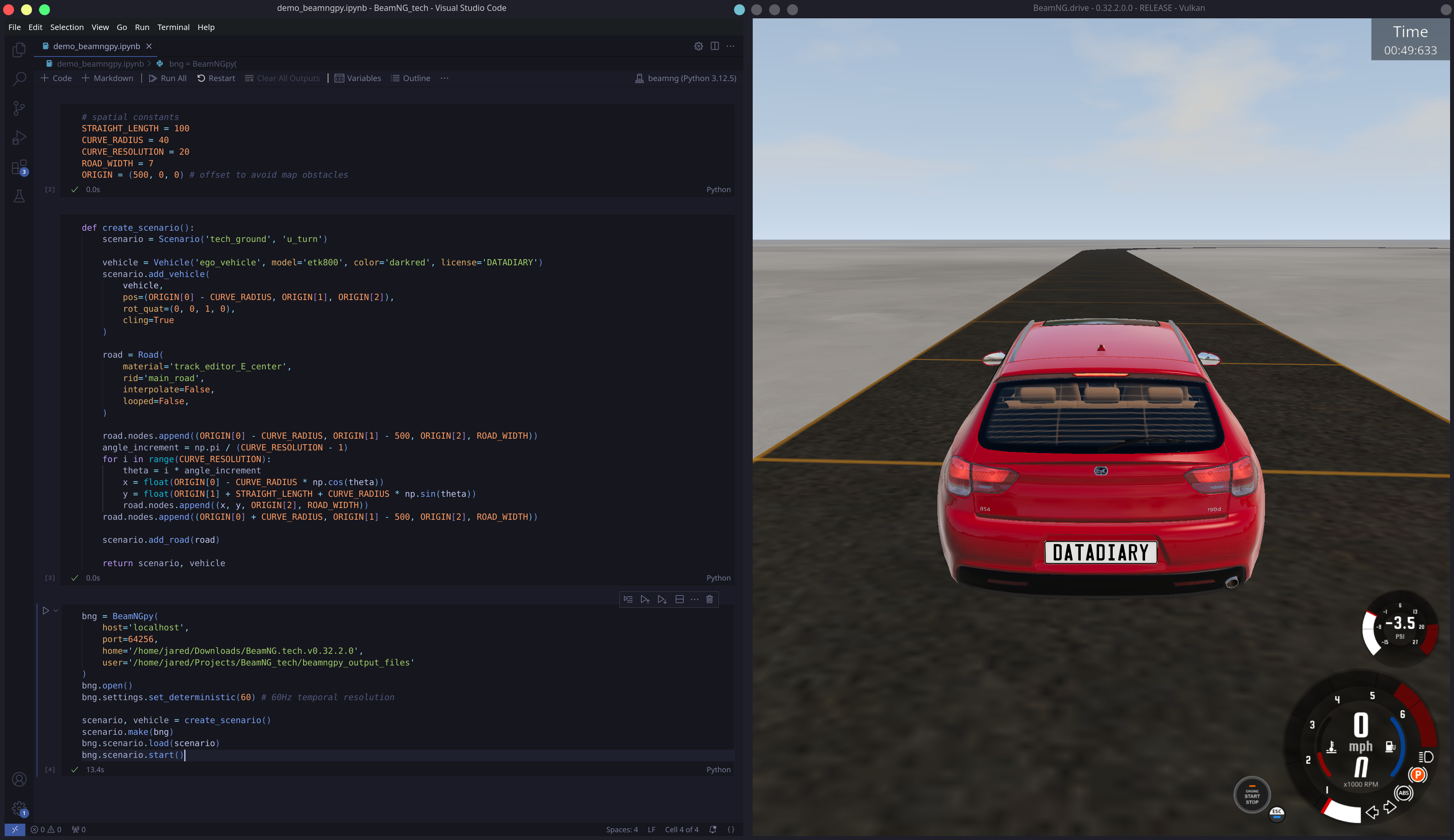
Let's go over the general plan. BeamNG allows us to poll the position, velocity, and orientation of the car as 3D Cartesian vectors (though we will discard $\hat{z}$). There is an implicit global origin and fixed basis. We need to leverage these vectors to calculate the 4 quantities that will feed into our control network. Two of the derivations are straightforward:

• $V_{err}$ : Subtract the magnitude of the velocity vector from the desired speed.
• $V_y$ (a.k.a. "drift") : Project the velocity vector onto the lateral component of the orientation vector.

$Y_{err}$ and $\Omega_{err}$ are a bit more complicated. We need to account for the non-uniform geometry of the U-turn. I propose a sliding origin, $O$, to streamline their derivation:

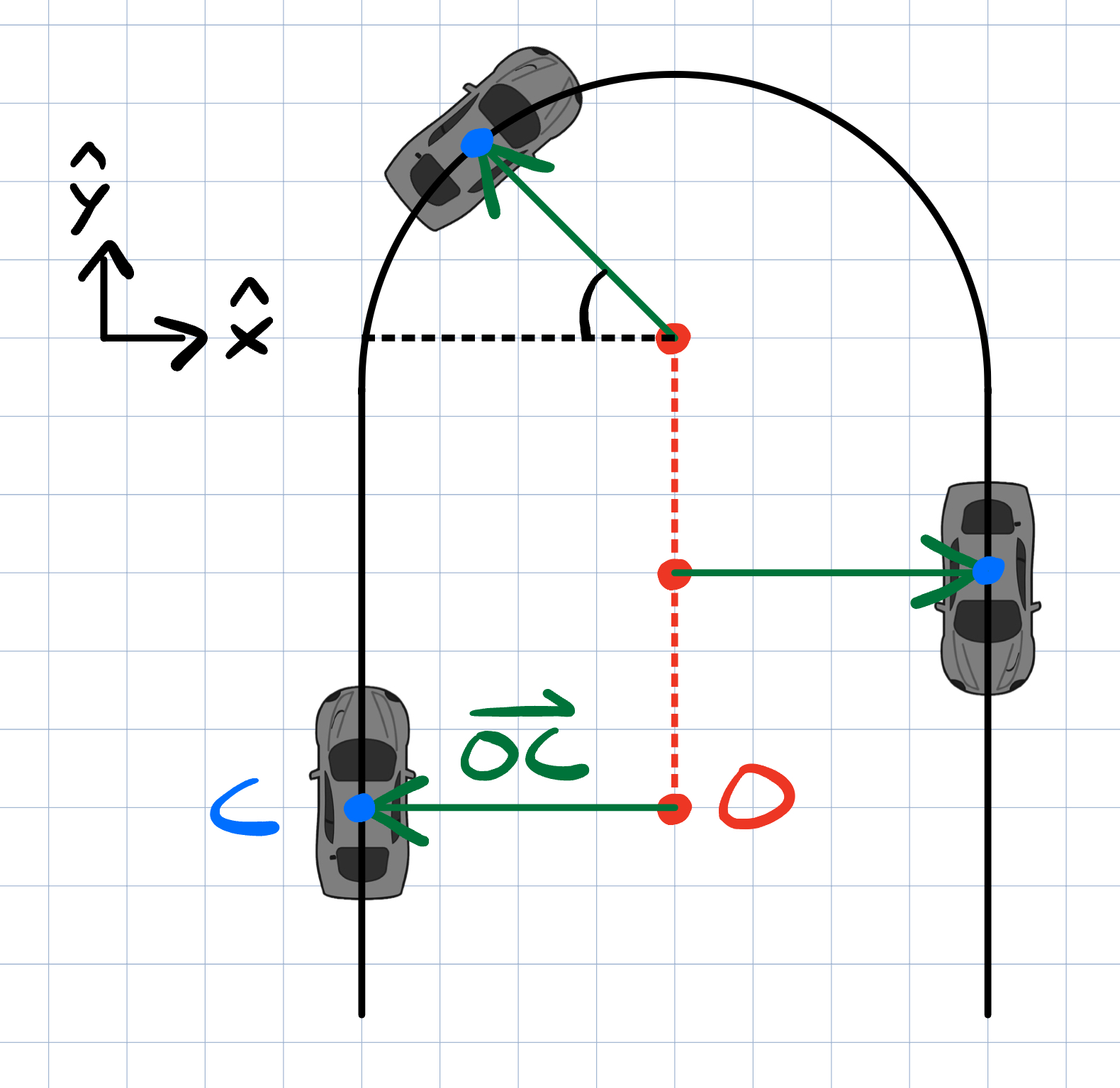
$O$ will be constrained to the U-turn's line of symmetry. It will track the car's vertical position up to the start of the U-turn, halt, then follow the car back down the final straight. We can draw a vector between this origin and the car, $\vec{OC}$. This vector will be the basis for the following location-agnostic logic for deriving the final 2 quantities:

• $Y_{err}$ : Subtract the radius of the U-turn from $|\vec{OC}|$.
• $\Omega_{err}$ : Rotate $\vec{OC}$ $\frac{\pi}{2}$ clockwise to get the car's target heading. Calculate the angle between the car's orientation and the target heading.

Now that we've figured out the measurements, it's important to clarify the structure of a 'trial'. Each trial will be a series of 10 episodes, where each episode starts the car at a slightly different angle. A variety of starting orientations ensures a robust evaluation of a given set of weights. Each episode will last 25 seconds, with a new measurement taken every quarter of a second. We will run 30 initial trials with random weights to give the surrogate function a solid introduction to the search space. We will then run 100 trials with the optimization loop described above.

Finally, we need a reward function. The authors propose a "negative weighted sum of normalized squared error values between the vehicle and the desired trajectory, including a = [steer, throttle] to penalize for abrupt actions":

We will simply calculate these quantities at each timestep, append them to a list, and perform the normalization and summation at the end of an episode.

Here's an outline of the code with some of the details abstracted as blackbox functions:

num_random_trials = 30
num_trials = 100
num_episodes_per_trial = 10
episode_duration = 25 # s
dt = 0.25 # s
target_speed = 16 # m/s
starting_angle = 140 # deg
 
def vehicle_control_network(weights, Y_err, V_err, V_y, Omega_err):
    steer = tanh(weights[8] * (
        weights[0] +
        weights[6] * (tanh(weights[1] * Y_err)) +
        weights[2] * Y_err +
        weights[3] * V_y +
        weights[4] * Omega_err +
        weights[7] * (tanh(weights[5] * Omega_err))
    ))
    throttle = tanh(weights[14] * (
        weights[9] +
        weights[10] * abs(Omega_err) +
        weights[11] * V_err +
        weights[13] * (tanh(weights[12] * V_err))
    ))
 
    return steer, throttle
 
def simulation_trial(weights):
    rewards = []
    for episode in range(num_episodes_per_trial):
        angle = starting_angle - (10 * episode)
        instantiate_vehicle(angle)
        
        quantities_list = []
        t = 0
        while t <= episode_duration:
            measurements = poll_vehicle_sensors()
            Y_err, V_err, V_y, Omega_err = derive_quantities(measurements)
            steer, throttle = vehicle_control_network(weights, Y_err, V_err, V_y, Omega_err)
            control_vehicle(steer, throttle)
            quantities_list.append([Y_err, V_err, V_y, Omega_err, steer, throttle])
 
            t += dt
        
        reward = weighted_normalized_squared_sum(quantities_list)
        rewards.append(reward)
 
    return mean(rewards)
 
optimizer = BayesianOptimization(f = simulation_trial)
optimizer.maximize(init_points = num_random_trials, n_iter = num_trials)

You can view the real code here.

Results

After roughly 12 hours, all 130 trials are complete. Let's have a look at the progression of the reward:

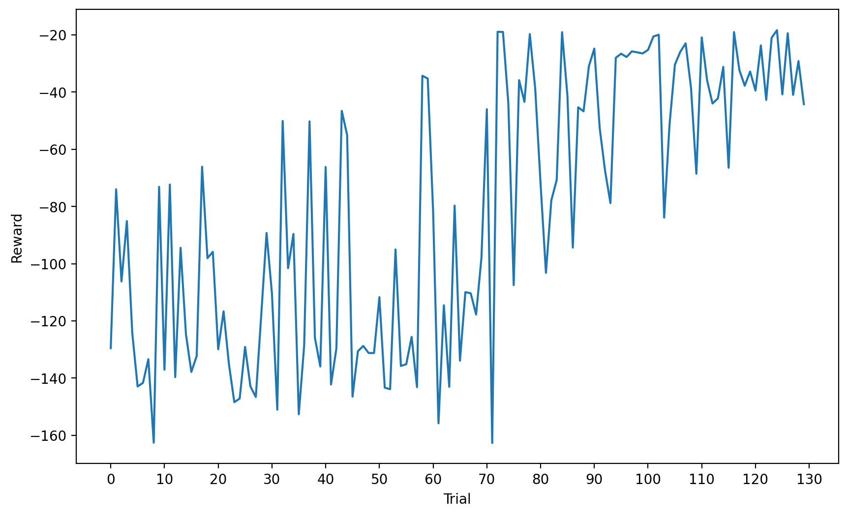
Quite unstable. Curiously, we see a jump in performance around the 70 trial mark. I anticipated consistent improvement after the first 30 trials. Let's visualize the actual trajectories of the car at some points on this curve:

A higher reward certainly seems to correspond to closer adherence to the track, but even the best trial shows persistent lateral deviation. Let's configure the car with the best set of weights and observe:

It appears that the car is properly incentivized to maintain the correct speed and orientation, but is never quite centered on the road.

We're on the right track (figuratively, if not literally) and I think we could improve by exploring the following ideas:

1. Tweaking the exploration-exploitation tradeoff parameter, $\xi$. The unstable improvement might be attributable to an over-emphasis on exploration.
2. Revising our normalization strategy. You'll recall that the reward function required a sum over normalized errors, where normalization entails shrinking a distribution of errors to range (-1, 1). The issue is that the maximum $Y_{err}$ can be massive. There's a choice to be made in preventing large errors from dominating the influence of small errors on the reward signal. I chose to cap the $Y_{err}$ at the distance equivalent to the radius of the U-turn, but a more sophisticated strategy might yield better results.

I may give these a try in a follow-up post, so be on the lookout!